KUKA-iiwa LBR14 Kinematics
Summary:
- 解IK,考虑冗余臂角,7-DOF S-R-S 构型位置IK解析解
文献[1]对于7自由度冗余仿人臂的逆运动学位置解做了很好的分析,主要考虑关节有位置限制时逆运动学解问题:
相关工作暂时不表,只记录求解过程和避免奇异的细节。
![]()
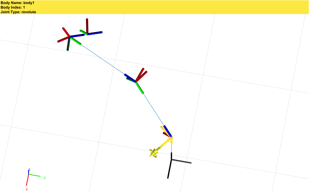
如图所示为常见的7-DOF机械臂,具有和人类相近的肩球关节和腕球关节以及肘部。
优点:和一般的6自由度机械臂相比,由于多了一个自由度,可以在保证末端位姿不变的情况下变换构型,达到避障、避免关节限幅(位置、速度、加速度),避免奇异,以及减小关节力矩消耗等作用。
缺点:自由度增加,串联系统的整体刚度下降,同时系统变得更加复杂(可能奇异的情况更多等等)。
一般的7自由度多为协作机械臂,也是利用上述特点达到工作中能够避免机械臂和接触到的人产生危险的碰撞等。
![]()
常见的比如KUKA的iiwa力控协作臂,还有安川的SDA10、ABB的yumi协作双臂等等,这些都满足S-R-S构型。
常见的操作都是人为加一个约束,通过调整约束参数同样能够得到解析解(Pieper’s Theorem: Closed-form solution always exists for any 6 dof robot with a spherical wrist)。
直接引出这篇文章的方法:
因为当末端tip位姿固定时,是能够求出肘关节的角度的(wrist, elbow, shoulder三点相对位置固定),那么通过引入三点所在的平面(Arm Plane),显然能够加入一个参数(臂角)
![]()
臂角参数一方面解决了冗余自由度的问题,另外一方面可以直接优化该参数来满足一些限制。
DH建模
\[\begin{array}{|c|c|c|c|c|}\hline i & {\theta_{i}} & {\alpha_{i}(\text { rad })} & {d_{i}} & {a_{i}} \\ \hline 1 & {\theta_{1}} & {-\pi / 2} & {d_{b s}} & {0} \\ {2} & {\theta_{2}} & {\pi / 2} & {d_{b s}} & {0} \\ {3} & {\theta_{2}} & {-\pi / 2} & {d_{s e}} & {0} \\ {4} & {\theta_{4}} & {\pi / 2} & {0} & {0} \\ {5} & {\theta_5} & {-\pi / 2} & {d_{e w}} & {0} \\ {6} & {\theta_{6}} & {\pi / 2} & {0} & {0} \\ {7} & {\theta_{7}} & {0} & {d_{w t}} & {0} \\ \hline\end{array}\]本文用的是标准的DH参数(一开始真没注意到,其实看表头a和d的下标就能看出来,改进型用的是i和i-1。
至于DH参数下细节可以参见另一篇文章
至于在计算Forward Kinematics时使用DH还是POE,其实都无所谓,DH优点是参数少(3n个描述结构,n个描述关节角),而PoE需要(6n个参数描述screw轴,n个描述关节角),但是PoE本质上并不需要Link的坐标系(和Joint重合了)。
总而言之,DH能干的事,PoE都能干,DH设计的目的是为了节约参数,仅此而已(还导致相邻关节平行会有奇异等等问题,导致了魔改版本加 \beta角)。
\[T_{i-1,i} = ^{i-1}T_{i}=\left(\operatorname{Rot}_{x_{i-1}}\left(\alpha_{i-1}\right) \cdot \operatorname{Trans}_{x_{i-1}}\left(a_{i-1}\right)\right) \cdot \left(\operatorname{Rot}_{z_{i}}\left(\theta_{i}\right) \cdot \operatorname{Trans}_{z_{i}}\left(d_{i}\right)\right) \\ M_i =\left(\operatorname{Rot}_{x_{i-1}}\left(\alpha_{i-1}\right) \cdot \operatorname{Trans}_{x_{i-1}}\left(a_{i-1}\right)\right) \cdot \operatorname{Trans}_{z_{i}}\left(d_{i}\right) \\ \operatorname{Rot}\left(\hat{\mathrm{z}}, \theta_{i}\right)=e^{\left[\mathcal{A}_{i}\right] \theta_{i}} \\ T_{0, n}=M_{1} e^{\left[\mathcal{A}_{1}\right] \theta_{1}} M_{2} e^{\left[\mathcal{A}_{2}\right] \theta_{2}} \cdots M_{n} e^{\left[\mathcal{A}_{n}\right] \theta_{n}} \\ = e^{\left[\mathcal{S}_{1}\right] \theta_{1}} \ldots e^{\left[\mathcal{S}_{n}\right] \theta_{n}} M\]因为每个joint的转动/平动都可以表示为[Ai],在joint坐标系内的screw又可以通过坐标变换(Ad)转换为{0}坐标系下的screw:
\[\left[\mathcal{S}_{b}\right]=T_{b a}\left[\mathcal{S}_{a}\right] T_{b a}^{-1} \\ \mathcal{S}_{b}=\mathrm{Ad}_{T_{b a}}\left(\mathcal{S}_{a}\right)\]因此只考虑FK计算末端的位姿的话,PoE貌似更方便?(感觉PoE的计算复杂度也并不是很高吗,本质上也还是齐次变换矩阵连乘,然后PoE的通用性会更加好一点)
\[e^{[\mathcal{S}] \theta}=\left[\begin{array}{cc}{e^{[\omega] \theta}} & {\left(I \theta+(1-\cos \theta)[\omega]+(\theta-\sin \theta)[\omega]^{2}\right) v} \\ {0} & {1}\end{array}\right] \\ (不考虑~~\omega = 0, ||v|| = 1) \\ e^{[\hat{\omega}]\theta} = I+sin{\theta}[\hat{\omega}] + (1-cos{\theta})[\hat{\omega}]^2 \\ = \left[\begin{array}{ccc}{\mathrm{c}_{\theta}+\hat{\omega}_{1}^{2}\left(1-\mathrm{c}_{\theta}\right)} & {\hat{\omega}_{1} \hat{\omega}_{2}\left(1-\mathrm{c}_{\theta}\right)-\hat{\omega}_{3} \mathrm{s}_{\theta}} & {\hat{\omega}_{1} \hat{\omega}_{3}\left(1-\mathrm{c}_{\theta}\right)+\hat{\omega}_{2} \mathrm{s}_{\theta}} \\ {\hat{\omega}_{1} \hat{\omega}_{2}\left(1-\mathrm{c}_{\theta}\right)+\hat{\omega}_{3} \mathrm{s}_{\theta}} & {\mathrm{c}_{\theta}+\hat{\omega}_{2}^{2}\left(1-\mathrm{c}_{\theta}\right)} & {\hat{\omega}_{2} \hat{\omega}_{3}\left(1-\mathrm{c}_{\theta}\right)-\hat{\omega}_{1} \mathrm{s}_{\theta}} \\ {\hat{\omega}_{1} \hat{\omega}_{3}\left(1-\mathrm{c}_{\theta}\right)-\hat{\omega}_{2} \mathrm{s}_{\theta}} & {\hat{\omega}_{2} \hat{\omega}_{3}\left(1-\mathrm{c}_{\theta}\right)+\hat{\omega}_{1} \mathrm{s}_{\theta}} & {\mathrm{c}_{\theta}+\hat{\omega}_{3}^{2}\left(1-\mathrm{c}_{\theta}\right)}\end{array}\right]\]个人认为FK中,为了通用性和易于理解,PoE>DH,至于别的地方,哪个好用用哪个吧~~
如果只是建立相对坐标的话,PoE的方法也更容易理解啊,而且也不难算 = =
Inverse Kinematics
在解决7-Dof机械臂SRS构型的逆解时,一般都用臂角(arm angle)来描述这个多出的自由度:
通过将\theta_3 初始化为0,然后根据建立臂角和\theta_3和其余关节的关系。
【注意】当\theta_3不动时,该机械臂其实已经退化为符合Pieper条件之一的6自由度臂(末端3轴交于1点)
这样无论是通过几何法还是分离末端位置和姿态矩阵,都能够得到逆解的方法:
\[T_{0,6}=T_{0,3}T_{3,6}\]当然使用旋量计算时同样能够利用该性质,这里先用几何法解释。
\[\begin{array}{l}{^{0} \boldsymbol{x}_{7}=^{0} l_{b s}+^{0} \boldsymbol{R}_{3}\left\{^{3} l_{s e}+^{3} \boldsymbol{R}_{4}\left(^{4} l_{e w}+^{4} \boldsymbol{R}_{7}^{7} l_{w t}\right)\right\}} \\ {^{0} \boldsymbol{R}_{7}=^{0} \boldsymbol{R}_{3}^{3} \boldsymbol{R}_{4}^{4} \boldsymbol{R}_{7}}\end{array}\]利用三角关系,以及肩到腕的距离x_sw,可列等式:
\[\begin{aligned}^{0} \boldsymbol{x}_{s w} &=^{0} \boldsymbol{x}_{7}-^{0} \boldsymbol{l}_{b s}-^{0} \boldsymbol{R}_{7} ~^{7} \boldsymbol{l}_{w t} \\ &=^{0} \boldsymbol{R}_{3}\left(^{3} \boldsymbol{l}_{s e}+^{3} \boldsymbol{R}_{4}^{4} \boldsymbol{l}_{e w}\right) \end{aligned}\]由于臂角变化时,肘关节并不变(三角形也不变),可以用臂角\phi和旋转轴来描述这个旋转矩阵:
\[^0 \boldsymbol{R}_{\psi}=\boldsymbol{I}_{3}+\sin \psi\left[^{0} \boldsymbol{u}_{s w} \times\right]+(1-\cos \psi)\left[^{0} \boldsymbol{u}_{s w} \times\right]^{2}\]因为是世界坐标系下的旋转(左乘),最终三角形上的link的{0}参考系下旋转矩阵可以描述为j3=0时的矩阵左乘臂角矩阵:
\[^0 \boldsymbol{R}_{4}=^{0} \boldsymbol{R}_{\psi}~^{0} \boldsymbol{R}_{4}^{ini} \\ ^0 \boldsymbol{R}_{3}=^{0} \boldsymbol{R}_{\psi}~^{0} \boldsymbol{R}_{3}^{ini} \\ 并且 ^{3}\boldsymbol {R}_{4} = ^{3}\boldsymbol{R}_{4}^{ini}\]肘角 Joint 4
\[\cos \theta_{4}=\frac{\left\|^{0} \boldsymbol{x}_{s w}\right\|^{2}-d_{s e}^{2}-d_{e w}^{2}}{2 d_{s e} d_{e w}} = \frac{\left\| ^{0} \boldsymbol{x}_{7}-^{0} \boldsymbol{l}_{b s}-^{0} \boldsymbol{R}_{7} ~^{7} \boldsymbol{l}_{w t} \right\|^{2}-d_{s e}^{2}-d_{e w}^{2}}{2 d_{s e} d_{e w}}\]肘角通常有两个解(正负)
Joint 1,2(决定末端位置) + 3 (决定臂角)
由于末端位置和姿态已知,可以轻松计算出x_sw在{0}系下的坐标
\[\begin{aligned}^{0} \boldsymbol{x}_{s w} &= ^{0}\boldsymbol{R}_{3}\left(^{3} \boldsymbol{l}_{s e}+^{3} \boldsymbol{R}_{4}^{4} \boldsymbol{l}_{e w}\right) \\ &= \left.^{0} \boldsymbol{R}_{1}^{ini} ~ ^{1}\boldsymbol{R}_{2}^{ini}~^{2} \boldsymbol{R}_{3}\right|_{\theta_{3}=0}\left(^{3} l_{s e}+^{3} \boldsymbol{R}_{4}~^{4} l_{e w}\right) \end{aligned}\]等式右侧未知量为两个,也即初始的\theta_1,\theta_2,该矩阵等式,可以解得初始的\theta_1,\theta_2以及初始的矩阵R_3^{ini}
\[~R_{0,3}^{ini}=\left[\begin{array}{ccc} {c_1c_2} & {- s_1} & {c_1s_2} \\ {s_1c_2} & {c_1} & {s_1s_2} \\ {-s_2} & {0} & {c_2}\end{array}\right]\]然后我们再规定臂角为已知,则可以求得对应臂角下的\theta_1,2,3:
\[^0 \boldsymbol{R}_{3}=^{0} \boldsymbol{R}_{\psi}~^{0} \boldsymbol{R}_{3}^{ini} \\ =\left(\boldsymbol{I}_{3} +\left[^{0} \boldsymbol{u}_{s w} \times\right]^{2} +\sin \psi\left[^{0} \boldsymbol{u}_{s w} \times\right]-\cos \psi\left[^{0} \boldsymbol{u}_{s w} \times\right]^{2} \right)~^{0} \boldsymbol{R}_{3}^{ini} \\ =\left(\left[^{0} \boldsymbol{u}_{s w}~^{0} \boldsymbol{u}_{s w}^T \right] +\sin \psi\left[^{0} \boldsymbol{u}_{s w} \times\right]-\cos \psi\left[^{0} \boldsymbol{u}_{s w} \times\right]^{2} \right)~^{0} \boldsymbol{R}_{3}^{ini} \\ =A_s sin{\psi} + B_s cos{\psi} + C_s\]右侧\phi假设已知,左侧未知量为\theta_1,\theta_2,\theta_3,则很容易求\theta_1,2,3,Paper上的Trans:
\[~^{0}R_{3}=\left[\begin{array}{ccc}{*} & {-\cos \theta_{1} \sin \theta_{2}} & {*} \\ {*} & {-\sin \theta_{1} \sin \theta_{2}} & {*} \\ {-\sin \theta_{2} \cos \theta_{3}} & {-\cos \theta_{2}} & {\sin \theta_{2} \sin \theta_{3}}\end{array}\right]\]【此处使用PoE的坐标】,计算FK验证通过,使用Matlab syms计算T03,发现也存在类似的能够计算的特点
\[R_{0,3}=\left[\begin{array}{ccc} {c_1c_2c_3 - s_1s_3} & {-c_1c_2s_3 - s_1c_3} & {c_1s_2} \\ {s_1c_2c_3 + c_1s_3} & {-s_1c_2s_3 + c_1c_3} & {s_1s_2} \\ {-c_3s_2} & {s_2s_3} & {c_2}\end{array}\right]\]Wrist(姿态计算Joint 5 6 7)
\[{^{0} \boldsymbol{R}_{7}=\boldsymbol{^{0}R}_{3}\boldsymbol{^{3}R}_{4}~ \boldsymbol{^{4}R}_{7}}\to \\\boldsymbol{^{4}R}_{7} = \boldsymbol{^{3}R}_{4}^T~\boldsymbol{^{0}R}_{3}^T ~\boldsymbol{^{0}R}_{7} \\=A_w sin{\psi} + B_w cos{\psi}+C_w \\A_w = \boldsymbol{^{3}R}_{4}^T~A_s^T ~\boldsymbol{^{0}R}_{7} \\B_w = \boldsymbol{^{3}R}_{4}^T~B_s^T ~\boldsymbol{^{0}R}_{7} \\C_w = \boldsymbol{^{3}R}_{4}^T~C_s^T ~\boldsymbol{^{0}R}_{7} \\\]由符号运算可以得到R_{4,7}关于\theta{5,6,7}的矩阵:
\[R_{4,7}=\left[\begin{array}{ccc} {c_5c_6c_7 - s_5s_7} & {-c_5c_6s_7 - s_5c_7} & {c_5s_6} \\ {-s_6c_7} & {s_6s_7} & {c_6} \\ {-s_5c_6c_7-c_5s_7} & {-c_5c_7+s_5c_6s_7} & {-s_5s_6}\end{array}\right]\]得到\theta{5,6,7}的计算公式(围绕R_47和Aw,Bw,Cw的矩阵等式进行计算)
最终,\theta1,2,3和\theta5,6,7均需要验算,修改正负号或者+pi满足矩阵完全相等。
![]()
图:Theta = [0.16, pi/2, 0.5, pi/3, 0.6,pi/6,0.3]的一组末端姿态对应的冗余解
IKforIIWA14(CartesianIIWA,-1,1,1,psi);
其中psi为输入的臂角。
![]()
![]()
Ik solver的精度得到验证的同时,也能看到在基本无关节奇异的情况下,各个关节只受到限幅的影响(+pi~-pi之间的跳变),而在某些情况下则有可能出现限幅范围内的跳变。
奇异以及Joint值函数关于臂角的变化
Singularity 在Chapt. II.E和Chapt. III.A中有详细的讨论:
大致可以按照tan, cos分为两类
a) tan, theta 1,3,5,7,求解公式大致相似:
\[\tan \theta_{i}=\frac{f_{n}(\psi)}{f_{d}(\psi)}\\ \begin{aligned} f_{n}(\psi) &=a_{n} \sin \psi+b_{n} \cos \psi+c_{n} \\ f_{d}(\psi) &=a_{d} \sin \psi+b_{d} \cos \psi+c_{d} \end{aligned}\]左右两边各求微分,可以得到\theta关于臂角的导数,从而能够发现导数始终存在
\[\frac{d \theta_{i}}{d \psi}=\frac{a_{t} \sin \psi+b_{t} \cos \psi+c_{t}}{f_{n}^{2}(\psi)+f_{d}^{2}(\psi)} \\ \begin{aligned} a_{t} &=b_{d} c_{n}-b_{n} c_{d} \\ b_{t} &=a_{n} c_{d}-a_{d} c_{n} \\ c_{t} &=a_{n} b_{d}-a_{d} b_{n} \end{aligned}\]对at,bt,ct的关系讨论,导数是否存在等于0的情况可以将theta1,3,5,7的值分为三种情况:
- 周期波动(存在不同的导数为0的解);
极大值和极小值在以上两个值取到。
- 单调(并在-pi~pi内无间断点)或者 两段单调(pi->-pi的穿越),此时导数始终不等于0;
- 两段单调单纯的加/减了pi),因为导数等于0只有重根,并且原值函数分子分母此时均为0,比较极限可以计算间断点两侧的tan(theta)是相同的,也就是只差了pi。
通过符号计算(利用at^2+bt^2 = ct^2以及sin(\psi),cos(\psi)和tan(\psi/2)的关系)分子分母均为0,同时不管是用罗必塔还是求极限,都能证明tan(\psi+\delta)在psi左右值相等,此时也对应肩或肘关节奇异。
\[\begin{array} f_{n}(\psi+\delta) &=a_{n} \sin (\psi+\delta)+b_{n} \cos (\psi+\delta) +c_{n} \\ &=a_{n} (\sin \psi \cos \delta + \cos \psi \sin \delta)+b_{n} (\cos\psi \cos\delta - \sin\psi \sin\delta) +c_{n} \\ &=\cos\delta(a_{n} \sin \psi+b_{n} \cos \psi+c_{n}) + c_n(1-\cos\delta) + \sin\delta(a_{n} \cos \psi-b_{n} \sin \psi) \\ &= 0 + c_{n}(1-\cos\delta)+\sin\delta (a_{n}\cdot\frac{(b_t-c_t)^2-a_t^2}{(b_t-c_t)^2+a_t^2} -b_{n}\cdot\frac{2a_{t}(b_t-c_t)}{(b_t-c_t)^2+a_t^2} ), using~a_{t}^2=c_t^2-b_t^2 \\ &=c_n(1-\cos\delta)+\sin\delta(\frac{(a_{t}b_{n}-a_{n}b_{t})(c_t-b_t)}{c_t(c_t-b_t)})\\ \to \tan{\theta_i} &= \frac{(1+\cos\delta)f_n(\psi)}{(1+\cos\delta)f_d(\psi)} \\ &=\frac{(1+\cos \delta)\left(a_{t} b_{n}-b_{t} a_{n}\right)+c_{t} c_{n} \sin \delta}{(1+\cos \delta)\left(a_{t} b_{d}-b_{t} a_{d}\right)+c_{t} c_{d} \sin \delta} \end{array}\\\]b) cos, theta2, 6
cos的正常情况是周期性波动,仅存在极少数奇异的情况(导数左右不连续,但是函数值连续),造成该情况的也是肩、肘的奇异。
\[\cos \theta_{i}=a \sin \psi+b \cos \psi+c \\ \frac{d \theta_{i}}{d \psi}=-\frac{1}{\sin \theta_{i}}(a \cos \psi-b \sin \psi)\]c) 对应肩/肘同时奇异的情况(theta2,6导数跳变,而theta1, 3, 5, 7会跳变)
下图中奇异出现在\psi等于0,左右侧的跳变不属于奇异,只是pi和-pi之间的切换。
同时\psi等于0附近的跳变可以通过切换state(一共有八组解:A4(正负),A1~3和A5~7各两组)来减少跳变。
此时IK的计算误差也比较大(Cartesian下误差范数到0.1左右(姿态误差较大,位置在0.01m以内)
![]()
![]()
奇异的情况下,还容易造成上图所示的跳帧现象(出现多解并且psi连续变化时,关节角不连续)
可以通过解空间的选择(2*2)来尽量规避这个问题,当然前提是需要知道当前的关节角(判断关节空间距离最近),然而当奇异的情况下,theta1,3,5,7可能无法计算(theta2,6=0导致矩阵出现大量0,之前求atan的方法肯定不好使了。一种可行的方法是判断当前Cartesian对应Shoulder或者Wrist已经奇异,并且psi也在奇异的点上时,使用附近的psi去逼近实际的关节角(或者直接用当前位置的关节角也行)。
%   at = bd * cn - bn * cd;
%   bt = an * cd - ad * cn;
%   ct = an * bd - ad * bn;
at = Bs(1,3) * Cs(2,3) - Bs(2,3) * Cs(1,3);
bt = As(2,3) * Cs(1,3) - As(1,3) * Cs(2,3);
ct = As(2,3) * Bs(1,3) - As(1,3) * Bs(2,3);

if(abs(at^2 + bt^2 - ct^2) < 1e-3 && abs(tan(phi / 2) - at / (bt - ct)) < 1e-3 )
    if(abs(theta2) > 1e-3)
        theta1 = atan((at * Bs(2,3) - bt * As(2,3)) / (at * Bs(1,3) - bt * As(1,3)));
    else
        theta1 = NaN;	% Singular at this psi.
    end
else
    theta1 = atan( (As(2,3) * sin(phi) + Bs(2,3)*cos(phi) + Cs(2,3)) / ...
    (As(1,3) * sin(phi) + Bs(1,3)*cos(phi) + Cs(1,3)));
end
![]()
因此需要对某个状态下的KUKA进行冗余度分析和冗余范围的确定:
关节限幅下的可行IK计算
留空…
REFERENCE
[1] Shimizu, M., Kakuya, H., Yoon, W. K., Kitagaki, K., & Kosuge, K. (2008). Analytical inverse kinematic computation for 7-DOF redundant manipulators with joint limits and its application to redundancy resolution. IEEE Transactions on Robotics, 24(5), 1131-1142.
[2] https://whtqh.github.io/blog/2019/10/03/DenavitHartenbergPara.html